Wk02: Project Management in RStudio and How R Thinks About Data
Learning objectives
- Be able to describe the different data types R uses
- Use c(), str(), class(), and typeof() to make and investigate vectors
- Understand coercion between data types
- Know how factors work under the hood
- Be able to manipulate factors
Videos
Project Management in RStudio
HOME is where I want to be
But I guess I’m
already there
I come home, a clean directory
I guess this must
be the place

Learning objectives
- Understand motivation for code and data management
- Know how to organize code, data, and results
- Know the basics of file paths and directory structures
- Be able to create and use an RStudio project
Working Directory and File Paths
Any time you’re working in R, R needs to know where you are within
your computer, which is referred to as the working directory.
The working directory could be something like
"YourUsername/Documents", or it could be something more
specific like "YourUsername/Documents/GradSchool/Chapter1".
Either way, R will think of everything in your computer as located
relative to your working directory. One of the nicest parts of using R
Projects is that they automatically set the working directory to the
folder containing the .RProject file. You can see your current working
directory by running the function getwd(), and you can set
it using setwd(), but if you’re using an R Project, you
generally shouldn’t mess with this too much.
All directories and files in R (and most computer languages) are
located using file paths. The two working directory examples we
just used are written as file paths, with / put between
different levels. Within YourUsername there is a folder
called Documents, and within that there is a folder called
GradSchool, and so on. In R, file paths are always wrapped
in quotes. There are 2 basic kinds of file paths: absolute and
relative. Absolute paths list out the full file path, usually
starting with your username, which you can also refer to using the
shortcut ~. So instead of
YourUsername/Documents, you can type
~/Documents. However, if you’ve got folders within folders
within folders, typing out absolute paths can get really tedious.
Relative paths are relative to your working directory.
So if R thinks we’re in that Chapter1 folder, and we want
to access a folder inside it called data, we can just type
data instead of
"YourUsername/Documents/GradSchool/Chapter1/data". What
happens if we need to go up a level, into GradSchool? Well
we can type .. to go up a level. So if we need to grab
something from our Chapter2 folder, but our working
directory is Chapter1, we would type
../Chapter2/FileWeWant.
Code & Data Organization
The scientific process is naturally incremental, and many projects start life as random notes, some code, then a manuscript, and eventually everything is a bit mixed together.
“Your greatest enemy is yourself four months ago” -Every grad student ever
A good project layout will ultimately make your life easier:
- It makes it easier to understand the pipeline from source data to final product
- It helps ensure the integrity of your data
- It makes it simpler to share your code with someone else
- It allows you to easily upload your code with your manuscript submission
- It makes it easier to pick the project back up after a break
Best practices for project organization
Although there is no “best” way to lay out a project, there are some general principles to adhere to that will make project management easier:
Treat raw data as read only
This is probably the most important goal of setting up a project. Raw
data should never be edited, because you can never be sure that you will
want to keep any edit you make, and you want to have a record of any
changes you make to data. Therefore, treat your raw data as “read only”,
perhaps even making a raw_data directory that is never
modified. If you do some data cleaning or modification, save the
modified file separate from the raw data, and ideally keep all the
modifying actions in a script so that you can review and revise them as
needed in the future.
Treat generated output as disposable
Anything generated by your scripts should be treated as disposable: it should all be able to be regenerated from your scripts. There are lots of different ways to manage this output, and what’s best may depend on the particular kind of project. At a minimum, it’s useful to have separate directories for each of the following:
- data: Ideally .csv files as these are flat, transparent, and universal. You may have other specialized formats as well. .rda and .rds are R-specific data files but you never need to use these.
- code (or script): .R files, perhaps .do files if Stata is your thing, .py files for Python, etc.
- results: .png or .pdf files for plots; .tex or .txt files for tables
- papers: .tex if you write in LaTeX, .doc for Word, .Rmd for RMarkdown, and .pdf or .html rendered documents.
RStudio Projects
As we learned last week, RStudio has a feature to help keep everything organized in a self-contained, reproducible package, called a “project”.
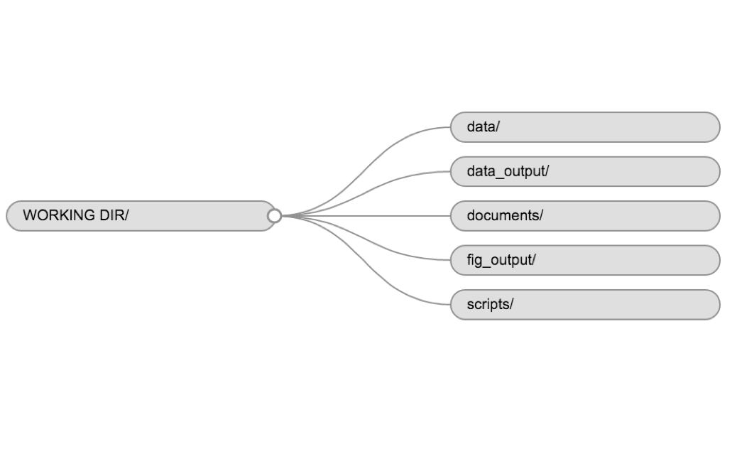
A project is a small file with a .Rproj extension, but
you can think of all the files and sub-directories as belonging to that
project. We recommend creating a directory and a project file for each
project you work on. It should look something like this:
Open the R Project file “R_DAVIS_20XX” you made for this class. You can do this by going to your file explorer (“Finder” on a Mac) and double clicking the file. Alternatively, you can open an existing project from within RStudio by clicking “File -> Open project…”, or by going to the top right with the blue R symbol and clicking your project from the drop-down menu.
Let’s now make a directory structure for your R_DAVIS_20XX project, using the structure described above: a folder for each of data, code, results, and papers. You can do this in RStudio by clicking on the “New Folder” button in the Files pane, or in your OS by navigating to the directory you just created.
Go up to the right hand corner of your screen and click the pull down tab that currently says R_DAVIS_20XX. Once you click it, you can toggle between multiple projects at once by clicking the white square/arrow icon next to the project name. This will allow you to have multiple projects open at once. If you want to switch projects completely, just click the project name (not the white square/arrow icon).
It is good to come up with some kind of naming convention that you can keep consistently (e.g. lastname_week_2.R).
How R Thinks About Data
Why Learn This Stuff?
It can be helpful to think of R, and your computer in general, as a collaborator who speaks a different language from you and is remarkably pedantic, but remarkably skilled as well. Learning a new language is difficult, and learning to speak it to an extremely literal and pedantic collaborator can make it even more frustrating. In such a collaboration, it might be useful to spend a little time learning the fundamentals of the language, understanding how you might interpret things differently, and not just rushing to “data data data!”
While this stuff might not be the most exciting material, or even feel useful right now, it is remarkably important in laying the groundwork for a fruitful collaboration with R. Skipping past this stuff and rushing to the finish line can leave you with a) error messages that don’t make sense to you, b) problems that are difficult to Google solutions to, and c) problems that R never even warns you about, because R didn’t think there was anything wrong!
All that being said, building a solid understanding of these fundamental ideas will save you headaches in the future, and leave you more well equipped to deal with new projects and concepts.
Vectors and data types
Vectors are the most basic way that R deals with data. A vector is
made up of a series of values, which could be numbers or characters.
Remember when we learned how to assign values to objects, like
x <- 5? Once we do that, x is a vector with a length of
1. Basically everything in R will be a vector or a bunch of vectors
bound together in some way, so knowing how vectors work is crucial to
working with more complex data structures.
We can bind together a series of values into a vector using the
c() function. For example we can create a vector of animal
weights and assign it to a new object weight_g:
weight_g <- c(50, 60, 65, 82)
weight_g
## [1] 50 60 65 82A vector can also contain characters:
animals <- c("mouse", "rat", "dog")
animals
## [1] "mouse" "rat" "dog"The quotes around “mouse”, “rat”, etc. are essential here. Without
the quotes R will assume there are objects called mouse,
rat and dog. As these objects don’t exist in
R’s memory, there will be an error message. You can use either single
' or double " quotes for characters.
There are many functions that allow you to inspect the content of a
vector. length() tells you how many elements are in a
particular vector:
length(weight_g)## [1] 4length(animals)## [1] 3An important feature of a vector is that all of the elements are the
same type of data. The function class() indicates the class
(the type of element) of an object:
class(weight_g)## [1] "numeric"class(animals)## [1] "character"The function str() provides an overview of the structure
of an object and its elements. It is a useful function when working with
large and complex objects.
str(weight_g)## num [1:4] 50 60 65 82str(animals)## chr [1:3] "mouse" "rat" "dog"A vector can be modified, adding values to the start or end of it.
You can use the c() function to add other elements to your
vector:
weight_g <- c(weight_g, 90) # add to the end of the vector
weight_g <- c(30, weight_g) # add to the beginning of the vector
weight_g
## [1] 30 50 60 65 82 90In the first line, we take the original vector weight_g,
add the value 90 to the end of it, and save the result back
into weight_g. Then we add the value 30 to the
beginning, again saving the result back into weight_g.
An atomic vector is the simplest R data
structure and is a linear vector of a single type. Above, we
saw 2 of the main atomic vector types that R uses:
"character" and "numeric" (or
"double"), which are numbers that can include decimals.
These are the basic building blocks that all R objects are built from.
There are 2 other atomic vector types that you’ll often
encounter:
"logical"forTRUEandFALSE(the boolean data type)"integer"for integer numbers (e.g.,2L, theLindicates to R that it’s an integer)
There are some other types, like complex and
raw but you’ll rarely, if ever, encounter them, so we won’t
go into them further.
You can check the type of your vector using the typeof()
function and inputting your vector as the argument.
typeof() is similar to class(), but it digs
even deeper down to the bare bones of how R thinks about data. The
difference is less important now, but we’ll come back around to it.
Challenge
We’ve seen that atomic vectors can be of type character, numeric (or double), integer, and logical. But what happens if we try to mix these types in a single vector?
What will happen in each of these examples? (hint: use
class()to check the data type of your objects):
num_char <- c(1, 2, 3, "a")
num_logical <- c(1, 2, 3, TRUE)
char_logical <- c("a", "b", "c", TRUE)
tricky <- c(1, 2, 3, "4")
Why do you think it happens?
How many values in
combined_logicalare"TRUE"(as a character) in the following example:
num_logical <- c(1, 2, 3, TRUE)
char_logical <- c("a", "b", "c", TRUE)
combined_logical <- c(num_logical, char_logical)- You’ve probably noticed that objects of different types get converted into a single, shared type within a vector. In R, we call converting objects from one class into another class coercion. These conversions happen according to a hierarchy, whereby some types get preferentially coerced into other types. Can you draw a diagram that represents the hierarchy of how these data types are coerced?
Subsetting vectors
If we want to extract one or several values from a vector, we must provide one or several indices in square brackets.
animals <- c("mouse", "rat", "dog", "cat")
animals[2] # could be read as "return the second value in animals"
## [1] "rat"animals[c(3, 2)] # could be read as "return the third and second values in animals"## [1] "dog" "rat"We can also repeat the indices to create an object with more elements than the original one:
animals[c(1, 2, 3, 2, 1, 4)]## [1] "mouse" "rat" "dog" "rat" "mouse" "cat"R indices start at 1. Programming languages like Fortran, MATLAB, Julia, and R start counting at 1, because that’s what human beings typically do. Languages in the C family (including C++, Java, Perl, and Python) count from 0 because that’s simpler for computers to do.
Conditional subsetting
Another common way of subsetting is by using a logical vector.
TRUE will select the element with the same index, while
FALSE will not:
weight_g <- c(21, 34, 39, 54, 55)
weight_g[c(TRUE, FALSE, TRUE, TRUE, FALSE)] # could be read as "give me the first value, not the second value, etc."
## [1] 21 39 54Typically, these logical vectors are not typed by hand, but are the output of other functions or logical tests. For instance, if you wanted to select only the values above 50:
weight_g > 50 # will return logicals with TRUE for the indices that meet the condition## [1] FALSE FALSE FALSE TRUE TRUE## so we can use this to select only the values above 50
weight_g[weight_g > 50]## [1] 54 55You can combine multiple tests using & (both
conditions are true, AND) or | (at least one of the
conditions is true, OR):
weight_g[weight_g < 30 | weight_g > 50]## [1] 21 54 55weight_g[weight_g >= 30 & weight_g == 21]## numeric(0)Here, < stands for “less than”, > for
“greater than”, >= for “greater than or equal to”, and
== for “equal to”. The double equal sign == is
a test for numerical equality between the left and right hand sides, and
should not be confused with the single = sign, which
performs variable assignment (similar to <-).
A common task is to search for certain strings in a vector. One could
use the “or” operator | to test for equality to multiple
values, but this can quickly become tedious. The function
%in% allows you to test if any of the elements of a search
vector are found:
animals <- c("mouse", "rat", "dog", "cat")
animals[animals == "cat" | animals == "rat"] # returns both rat and cat
## [1] "rat" "cat"animals %in% c("rat", "cat", "dog", "duck", "goat")## [1] FALSE TRUE TRUE TRUEanimals[animals %in% c("rat", "cat", "dog", "duck", "goat")]## [1] "rat" "dog" "cat"Challenge
- Can you figure out why
"four" > "five"returnsTRUE?
Hint: If you wanted to sort a collection of words, what would you hope R would do?
Vector Math and Recycling
You can do basic mathematical operations with vectors in R. We won’t get into this too deeply, but you should be aware of how R approaches these operations.
You can add a number to a vector of numbers like this:
x <- 1:10

x + 3
## [1] 4 5 6 7 8 9 10 11 12 13Or multiply all the values in a vector by a number:
x * 10## [1] 10 20 30 40 50 60 70 80 90 100By default, R will do value-by-value math. So if you add together two vectors of equal length, R will return a vector of the 1st value of each added together, then the 2nd value of each added together, etc. Let’s take a look here:
y <- 100:109

x + y
## [1] 101 103 105 107 109 111 113 115 117 119As you can see, the first entry we get back is 1 + 100, the second is 2 + 101, and so on. What happens if we try to add two vectors that aren’t the same length?
z <- 1:2

x + z
## [1] 2 4 4 6 6 8 8 10 10 12Whoa… what happened here? R does something called
recycling. It adds together the first values of each
vector, then the second values, but then it runs out of values in vector
z. It then recycles the values of z, so it will add the
3rd value of x to the 1st value of z, then the 4th value of x to the 2nd
value of z, and so on. Essentially, it recycles z from 1,2
into 1,2,1,2,1,2,1,2,1,2, then does the addition.
We actually already saw this behavior: when we added 3 to x, 3 gets recycled into a vector of 3s that is the same length as x.
Since the length of x is 10, it is a multiple of the length of z, which is 2. What happens if the longer vector isn’t a multiple of the shorter one?
z <- 1:3

x + z
## Warning in x + z: longer object length is not a multiple of shorter object
## length## [1] 2 4 6 5 7 9 8 10 12 11a <- x + z## Warning in x + z: longer object length is not a multiple of shorter object
## lengthR warns us about this! However, if you try to assign this result to
an object, we get the warning, but the assignment works. z will get
recycled until it reaches the length of x. So z gets recycled from being
1,2,3 to being 1,2,3,1,2,3,1,2,3,1, then gets
added to x. This can give you unexpected results if you’re doing math
with vectors and you’re not paying attention to what’s going on.
Recycling also happens with logical vectors:
x[c(TRUE, FALSE)]## [1] 1 3 5 7 9x[c(TRUE, FALSE, FALSE)]## [1] 1 4 7 10As mentioned earlier, logical vectors are often generated as intermediate steps when we’re subsetting. If you’re not careful about the lengths of these intermediate logical vectors, you can get some funky results without even noticing how they happened.
Missing data
As R was designed to analyze datasets, it includes the concept of
missing data (which is uncommon in other programming languages). Missing
data are represented in vectors as NA.
When doing operations on numbers, most functions will return
NA if the data you are working with include missing values.
This feature makes it harder to overlook the cases where you are dealing
with missing data. You can add the argument na.rm=TRUE to
calculate the result while ignoring the missing values.
heights <- c(2, 4, 4, NA, 6)
mean(heights)
## [1] NAmax(heights)## [1] NAmean(heights, na.rm = TRUE)## [1] 4max(heights, na.rm = TRUE)## [1] 6If your data include missing values, you may want to become familiar
with the functions is.na(), na.omit(), and
complete.cases(). See below for examples.
## Extract those elements which are not missing values.

is.na(heights) # this returns a logical vector with TRUE where there is an NA
## [1] FALSE FALSE FALSE TRUE FALSE!is.na(heights) # the ! means "is not", so now we get a logical vector with FALSE for NAs## [1] TRUE TRUE TRUE FALSE TRUEheights[!is.na(heights)] # now we put that logical vector in, and it will NOT return the entries with NA## [1] 2 4 4 6## Extract those elements which are complete cases. The returned object is an atomic vector of type `"numeric"` (or `"double"`).
heights[complete.cases(heights)]## [1] 2 4 4 6Recall that you can use the typeof() function to find
the type of your atomic vector.
Challenge
- Using this vector of heights in inches, create a new vector with the NAs removed.
heights <- c(63, 69, 60, 65, NA, 68, 61, 70, 61, 59, 64, 69, 63, 63, NA, 72, 65, 64, 70, 63, 65)- Use the function
median()to calculate the median of theheightsvector. - Use R to figure out how many people in the set are taller than 67 inches.
Other Data Structures
Vectors are one of the many data structures that R
uses. Other important ones are lists (list), data frames
(data.frame), matrices (matrix), arrays
(array), and factors (factor). These are all
built from combinations of vectors, so much of what you learned about
vectors will be important when working with these data structures.
Lists
Lists are the most fundamental way that R works with multiple vectors. A list is simply a bunch of vectors put together. The vectors can be different data types, so a list could hold a character vector with the names of your sampling sites as well as a numeric vector with their percent tree cover.
Lists are extremely flexible, and you’ll come across them a lot in various shapes and sizes. We’ll talk about them a bit more in later lessons.
Data Frames
Data frames are the most common way we work with tabular data in R. Data frames at their core are just picky lists. A data frame is a list where every vector has to be the same length, which is akin to every column having the same number of rows. This means a data frame is rectangular, which is why it matches up with tabular data we’re used to working with. A list could have one vector that has 5 values and one vector that has a thousand.
Matrices and Arrays
Matrices (2D) and Arrays (3D or more) are similar to dataframes and lists, but they are a little more barebones. Matrices and arrays must be made of a single type of data, no mixing types across different columns like in a dataframe. We won’t work with these much, but you might encounter them if you do something like population modeling in R. If you remember your basics of vectors, you should be pretty well equipped to tackle matrices and arrays.
Factors
Factors are a bit funky, and they can be equally useful and frustrating. Factors look a lot like 1-dimensional character vectors, but they behave a bit differently.
Factors are used to represent categorical data. Let’s make one to play around with:
sex <- factor(c("male", "female", "female", "male"))
class(sex)
## [1] "factor"If we ask for the class of sex, we see that it’s a factor. Let’s try
using typeof(), which goes a little deeper:
typeof(sex)## [1] "integer"An integer???
Factors are really just integer vectors with character labels attached to them.
Once created, factors can only contain a pre-defined set of values,
known as levels. By default, R always sorts levels in
alphabetical order. For instance, in our sex factor, R will
assign the integer 1 to the level "female" and
2 to the level "male" (becausef
comes before m, even though the first value in
sex is "male"). You can see this by using the
function levels() and you can find thenumber of levels
using nlevels():
levels(sex)## [1] "female" "male"nlevels(sex)## [1] 2Sometimes, the order of the factors does not matter, other times you
might want to specify the order because it is meaningful (e.g., “low”,
“medium”, “high”), it improves your visualization, or it is required by
a particular type of analysis. Here, one way to reorder our levels in
the sex vector would be:
sex # current order## [1] male female female male
## Levels: female malesex <- factor(sex, levels = c("male", "female"))
sex # after re-ordering## [1] male female female male
## Levels: male femaleIn R’s memory, these factors are represented by integers (1, 2, 3),
but are more informative than integers because factors are self
describing: "female", "male" is more
descriptive than 1, 2. Which one is “male”?
You wouldn’t be able to tell just from the integer data. Factors, on the
other hand, have this information built in. It is particularly helpful
when there are many levels (like the species names in our example
dataset).
Converting factors
If you need to convert a factor to a character vector, you use
as.character(x).
as.character(sex)## [1] "male" "female" "female" "male"Converting factors where the levels appear as numbers (such as
concentration levels, or years) to a numeric vector is a little
trickier. The as.numeric() function returns the index
values of the factor, not its levels, so it will result in an entirely
new (and unwanted in this case) set of numbers. One method to avoid this
is to convert factors to characters, and then to numbers.
year_fct <- factor(c(1990, 1983, 1977, 1998, 1990))
as.numeric(year_fct)               # Wrong! And there is no warning...
## [1] 3 2 1 4 3as.numeric(as.character(year_fct)) # This does the trick## [1] 1990 1983 1977 1998 1990Renaming factors
You can rename the levels using the levels()
function
levels(sex)## [1] "male" "female"levels(sex)[1]## [1] "male"levels(sex)[1] <- "MALE"
sex## [1] MALE female female MALE
## Levels: MALE femalelevels(sex) <- c("MALE", "FEMALE")
sex## [1] MALE FEMALE FEMALE MALE
## Levels: MALE FEMALEChallenge
- Copy, paste and run the code below in your R script:
treatment <- factor(c("high", "low", "low", "medium", "high")) - First, re-order the levels of
treatmentso that “low” is first, “medium” is second, and “high” is third. Hint: Use thefactor()function again, but with an additionallevelsargument. - Next, check the names with the
levels()function, then use this same function to rename the levels of treatment to “L”, “M” and “H”
ANSWER
treatment <- factor(c("high", "low", "low", "medium", "high"))
treatment <- factor(treatment, levels = c("low", "mediam", "high"))
levels(treatment) <- c("L", "M", "H")
treatment
## [1] H L L <NA> H
## Levels: L M HWhy Factors?
Factors can be convenient at times, and they will pop up pretty frequently, but in most circumstances, character strings will give you fewer hassles. It’s usually best to start with character vectors, and convert them explicitly to factors if you need to.
Some functions in R will automatically convert character strings to
factors. For instance, read.csv() run in older versions R
will turn any character data into factors, while in newer versions this
has been changed to keep them as characters. If you aren’t sure, you can
use the argument stringsAsFactors=FALSE in
read.csv() to make sure your character strings as character
strings.
This lesson is adapted from Data Carpentry’s Ecology Workshop Introduction to R