Wk05: Manipulating and analyzing data in the tidyverse, Part 2
Learning objectives
- Use conditional statements to create new variables in a dataframe
- Use
joinfunctions to join two dataframes together - Describe the concept of a wide and a long table format and for which purpose those formats are useful.
- Reshape a data frame from long to wide format and back with the
pivot_widerandpivot_longercommands from thetidyrpackage.
Videos
- Data manipulation Part 2a: Conditionals
- Data manipulation Part 2b: Joins
- Data manipulation Part 2c: Pivots and Exporting Data
- Video Discussion
Conditional Statements
When working with your data, you may want to create a new variable in a data frame, but only if a certain conditions are true. Conditional statements are a series of logical conditions that can help you manipulate your data to create new variables.
We’ll begin again with our surveys data, and remember to load in the tidyverse
library(tidyverse)
surveys <- read_csv("https://ucd-rdavis.github.io/R-DAVIS/data/portal_data_joined.csv")
The general logic of conditional statements is this: if a statement is true, then execute x, if it is false, then execute y. For example, let’s say that we want to create a categorical variable for hindfoot length in our data. Using the summary function below, we see that the mean hindfoot length is 29.29, so let’s split the data at the mean using a conditional statement.
summary(surveys$hindfoot_length)## Min. 1st Qu. Median Mean 3rd Qu. Max. NA's
## 2.00 21.00 32.00 29.29 36.00 70.00 4111ifelse() function
To do this, we define the logic: if hindfoot length is less than the
mean of 29.29, assign “small” to this new variable, otherwise, assign
“big” to this new variable. We can call this hindfoot_cat
to specify the categorical variable. We will first do this using the
ifelse() function, where the first argument is a TRUE/FALSE
statement, the second argument is the new variable if the statement is
true, and the third argument is the new variable if the statement is
false.
surveys$hindfoot_cat <- ifelse(surveys$hindfoot_length < 29.29, "small", "big")
head(surveys$hindfoot_cat)
## [1] "big" "big" "big" "big" "big" "small"case_when() function
The tidyverse provides a way to integrate conditional statements by
combining mutate() with the conditional function:
case_when(). This function uses a series of two-sided
formulas where the left-hand side determines describes the condition,
and the right supplies the result. The final condition should always be
TRUE, meaning that when the previous conditions have not been met,
assign the last value. Using this function we can re-write the
hindfoot_cat variable using the tidyverse.
A note: Always be cautious about what might be left out when naming
the conditions. In the previous ifelse() example we saw
that NAs in the data remained NAs in the new variable construction.
However, this is not so when using case_when(). Instead,
this function takes the last argument to mean “anything that is left”
rather than hindfoot_length > 29.29 == F. So when we run the
equivalent conditions in this function, it assigns “small” where
hindfoot_lengths are NA.
surveys %>%
  mutate(hindfoot_cat = case_when(
    hindfoot_length > 29.29 ~ "big",
    TRUE ~ "small"
  )) %>%
  select(hindfoot_length, hindfoot_cat) %>%
  head()
## # A tibble: 6 × 2
## hindfoot_length hindfoot_cat
## <dbl> <chr>
## 1 32 big
## 2 33 big
## 3 37 big
## 4 36 big
## 5 35 big
## 6 14 smallTo adjust for this, we need to add in more than one condition:
surveys %>%
  mutate(hindfoot_cat = case_when(
    hindfoot_length > 29.29 ~ "big",
    is.na(hindfoot_length) ~ NA_character_,
    TRUE ~ "small"
  )) %>%
  select(hindfoot_length, hindfoot_cat) %>%
  head()
## # A tibble: 6 × 2
## hindfoot_length hindfoot_cat
## <dbl> <chr>
## 1 32 big
## 2 33 big
## 3 37 big
## 4 36 big
## 5 35 big
## 6 14 smallChallenge
Using the iris data frame (this is built in to R),
create a new variable that categorizes petal length into three
groups:
- small (less than or equal to the 1st quartile)
- medium (between the 1st and 3rd quartiles)
- large (greater than or equal to the 3rd quartile)
Hint: Explore the iris data using
summary(iris$Petal.Length), to see the petal length
distribution. Then use your function of choice: ifelse() or
case_when() to make a new variable named
petal.length.cat based on the conditions listed above. Note
that in the iris data frame there are no NAs, so we don’t
have to deal with them here.
ANSWER
iris$petal.length.cat <- ifelse(iris$Petal.Length <= 1.6, "low",
                          ifelse(iris$Petal.Length > 1.6 &
                                   iris$Petal.Length < 5.1, "medium",
                           "high"))

iris %>%
  mutate(
    petal.length.cat = case_when(
      Petal.Length <= 1.6 ~ "small",
      Petal.Length > 1.6 & Petal.Length < 5.1 ~ "medium",
      TRUE ~ "large")) %>%
  head()
## Sepal.Length Sepal.Width Petal.Length Petal.Width Species petal.length.cat
## 1 5.1 3.5 1.4 0.2 setosa small
## 2 4.9 3.0 1.4 0.2 setosa small
## 3 4.7 3.2 1.3 0.2 setosa small
## 4 4.6 3.1 1.5 0.2 setosa small
## 5 5.0 3.6 1.4 0.2 setosa small
## 6 5.4 3.9 1.7 0.4 setosa mediumJoining two dataframes
Often when working with real data, data might be separated in
multiple .csvs. The join family of dplyr functions can
accomplish the task of uniting disparate data frames together rather
easily. There are many kind of join functions that dplyr
offers, and today we are going to cover the most commonly used function
left_join.
To learn more about the join family of functions, check
out this useful
link.
Let’s read in another dataset. This data set is a record of the tail
length of the rodents in our surveys dataframe. For some
annoying reason, it was recorded on a seperate data sheet. We want to
take the tail length data and add it to our surveys dataframe.
tail <- read_csv("https://ucd-rdavis.github.io/R-DAVIS/data/tail_length.csv")The join functions join dataframes together based on
shared columns between the two data frames. Let’s see what the
tail data frame looks like.
str(tail)## spc_tbl_ [34,786 × 2] (S3: spec_tbl_df/tbl_df/tbl/data.frame)
## $ record_id : num [1:34786] 1 72 224 266 349 363 435 506 588 661 ...
## $ tail_length: num [1:34786] 8.46 6.27 7.47 6.45 8.06 ...
## - attr(*, "spec")=
## .. cols(
## .. record_id = col_double(),
## .. tail_length = col_double()
## .. )
## - attr(*, "problems")=<externalptr>Looks like we have a data frame with 34,786 rows and two columns:
record_id and tail_length. Luckily, both our
surveys and tail data frames have the column
record_id. We can use this shared column to
join the two data frames together.
The basic structure of a join looks like this:
join_type(TableA, TableB, by=columnTojoinBy)
There are many different kinds of join types:
inner_joinwill return all the rows from Table A that has matching values in Table B, and all the columns from both Table A and Bleft_joinreturns all the rows from Table A with all the columns from both A and B. Rows in Table A that have no match in Table B will return NAsright_joinreturns all the rows from Table B and all the columns from table A and B. Rows in Table B that have no match in Table A will return NAs.full_joinreturns all the rows and all the columns from Table A and Table B. Where there are no matching values, returns NA for the one that is missing.
For our data we are going to use a left_join. We want
all the rows from the surveys data frame, and we want all
the columns from both data frames to be in our new data frame.
You might have noticed that our tail data frame had
fewer rows than our surveys data frame. We must not have
tail length measurements for all of our observations in
surveys. Since we are using a left_join, any
observations in surveys that do not have a match in
tail will be given an NA value for
tail_length.
surveys_joined <- left_join(surveys, tail, by = "record_id")If we don’t include the by = argument, the default is to
join by all the variables with common names across the two data frames.
Let’s take a look at our new surveys_joined data frame:
str(surveys_joined)## spc_tbl_ [35,549 × 15] (S3: spec_tbl_df/tbl_df/tbl/data.frame)
## $ record_id : num [1:35549] 1 2 3 4 5 6 7 8 9 10 ...
## $ month : num [1:35549] 7 7 7 7 7 7 7 7 7 7 ...
## $ day : num [1:35549] 16 16 16 16 16 16 16 16 16 16 ...
## $ year : num [1:35549] 1977 1977 1977 1977 1977 ...
## $ plot_id : num [1:35549] 2 3 2 7 3 1 2 1 1 6 ...
## $ species_id : chr [1:35549] "NL" "NL" "DM" "DM" ...
## $ sex : chr [1:35549] "M" "M" "F" "M" ...
## $ hindfoot_length: num [1:35549] 32 33 37 36 35 14 NA 37 34 20 ...
## $ weight : num [1:35549] NA NA NA NA NA NA NA NA NA NA ...
## $ genus : chr [1:35549] "Neotoma" "Neotoma" "Dipodomys" "Dipodomys" ...
## $ species : chr [1:35549] "albigula" "albigula" "merriami" "merriami" ...
## $ taxa : chr [1:35549] "Rodent" "Rodent" "Rodent" "Rodent" ...
## $ plot_type : chr [1:35549] "Control" "Long-term Krat Exclosure" "Control" "Rodent Exclosure" ...
## $ hindfoot_cat : chr [1:35549] "big" "big" "big" "big" ...
## $ tail_length : num [1:35549] 8.46 8.31 10.08 7.4 7.78 ...
## - attr(*, "spec")=
## .. cols(
## .. record_id = col_double(),
## .. month = col_double(),
## .. day = col_double(),
## .. year = col_double(),
## .. plot_id = col_double(),
## .. species_id = col_character(),
## .. sex = col_character(),
## .. hindfoot_length = col_double(),
## .. weight = col_double(),
## .. genus = col_character(),
## .. species = col_character(),
## .. taxa = col_character(),
## .. plot_type = col_character()
## .. )
## - attr(*, "problems")=<externalptr>We now have a new data frame called surveys_joined which
has all of the information from our original surveys data
frame, plus the new tail_length column that we added when
joining the tail data frame.
Challenge
- Filter the data so that only species_id = NL,and call this
surveysNL
- Join the
taildata to thesurveysNLdata (i.e. left join withsurveysNLon the left). Name itsurveysNL_tail_left. How many rows are there?
- Join the
surveysNLdata to thetail data(i.e. right join withsurveysNLon the left). Name itsurveysNL_tail_right. How many rows are there?
ANSWER
# 1.
surveysNL <- surveys %>%
  filter(species_id == "NL") #filter to just the species NL

# 2.
surveysNL_tail_left <- left_join(surveysNL, tail, by = "record_id") #a new column called tail_length was added
nrow(surveysNL_tail_left)
## [1] 1252# 3.
surveysNL_tail_right <- right_join(surveysNL, tail, by = "record_id") #a new column called tail_length was added
nrow(surveysNL_tail_right)## [1] 34786Reshaping with pivot functions
In the spreadsheet lesson we discussed how to structure our data leading to the four rules defining a tidy dataset:
- Each variable has its own column
- Each observation has its own row
- Each value must have its own cell
- Each type of observational unit forms a table
Here we examine the fourth rule: Each type of observational unit forms a table.
In surveys , the rows of surveys contain
the values of variables associated with each record (the unit), values
such the weight or sex of each animal associated with each record. What
if instead of comparing records, we wanted to compare the different mean
weight of each species between plots?
We’d need to create a new table where each row (the unit) is comprise
of values of variables associated with each plot. In practical terms
this means the values of the species in species would
become the names of column variables and the cells would contain the
values of the mean weight observed on each plot.
Having created a new table, it is therefore straightforward to explore the relationship between the weight of different species within, and between, the plots. The key point here is that we are still following a tidy data structure, but we have reshaped the data according to the observations of interest: average species weight per plot instead of recordings per date.
The opposite transformation would be to transform column names into values of a variable.
We can do both these of transformations with two new
tidyr functions, pivot_longer() and
pivot_wider().
pivot_wider
pivot_wider() widens data by increasing the
number of columns and decreasing the number of rows. It takes
three main arguments:
- the data
names_fromthe name of the column you’d like to spread outvalues_fromthe data you want to fill all your new columns with
Let’s try an example using our surveys data. Let’s pretend we are interested in what the mean weight is for each species in each plot. How would we create a dataframe that would tell us that information?
First, we need to calculate the mean weight for each species in each plot:
surveys_mz <- surveys %>%
  filter(!is.na(weight)) %>%
  group_by(species_id, plot_id) %>%
  summarize(mean_weight = mean(weight))
## `summarise()` has grouped
## output by 'species_id'. You can
## override using the `.groups`
## argument.str(surveys_mz) #let's take a look at the data## gropd_df [382 × 3] (S3: grouped_df/tbl_df/tbl/data.frame)
## $ species_id : chr [1:382] "BA" "BA" "BA" "BA" ...
## $ plot_id : num [1:382] 1 2 3 5 18 19 20 21 1 2 ...
## $ mean_weight: num [1:382] 7 6 8.61 7.75 9.5 ...
## - attr(*, "groups")= tibble [25 × 2] (S3: tbl_df/tbl/data.frame)
## ..$ species_id: chr [1:25] "BA" "DM" "DO" "DS" ...
## ..$ .rows : list<int> [1:25]
## .. ..$ : int [1:8] 1 2 3 4 5 6 7 8
## .. ..$ : int [1:24] 9 10 11 12 13 14 15 16 17 18 ...
## .. ..$ : int [1:23] 33 34 35 36 37 38 39 40 41 42 ...
## .. ..$ : int [1:22] 56 57 58 59 60 61 62 63 64 65 ...
## .. ..$ : int [1:24] 78 79 80 81 82 83 84 85 86 87 ...
## .. ..$ : int [1:23] 102 103 104 105 106 107 108 109 110 111 ...
## .. ..$ : int [1:24] 125 126 127 128 129 130 131 132 133 134 ...
## .. ..$ : int [1:6] 149 150 151 152 153 154
## .. ..$ : int [1:23] 155 156 157 158 159 160 161 162 163 164 ...
## .. ..$ : int [1:24] 178 179 180 181 182 183 184 185 186 187 ...
## .. ..$ : int [1:23] 202 203 204 205 206 207 208 209 210 211 ...
## .. ..$ : int [1:9] 225 226 227 228 229 230 231 232 233
## .. ..$ : int [1:3] 234 235 236
## .. ..$ : int [1:11] 237 238 239 240 241 242 243 244 245 246 ...
## .. ..$ : int [1:24] 248 249 250 251 252 253 254 255 256 257 ...
## .. ..$ : int [1:24] 272 273 274 275 276 277 278 279 280 281 ...
## .. ..$ : int [1:2] 296 297
## .. ..$ : int [1:17] 298 299 300 301 302 303 304 305 306 307 ...
## .. ..$ : int [1:24] 315 316 317 318 319 320 321 322 323 324 ...
## .. ..$ : int [1:6] 339 340 341 342 343 344
## .. ..$ : int [1:2] 345 346
## .. ..$ : int [1:10] 347 348 349 350 351 352 353 354 355 356
## .. ..$ : int [1:16] 357 358 359 360 361 362 363 364 365 366 ...
## .. ..$ : int [1:8] 373 374 375 376 377 378 379 380
## .. ..$ : int [1:2] 381 382
## .. ..@ ptype: int(0)
## ..- attr(*, ".drop")= logi TRUEIn surveys_mz there are 382 rows and 3 columns. Using
pivot_wider we are going to increase the number of
columns and decrease the number of rows. We want each row to
signify a single species, with their mean weight listed for each plot
id. How many rows do we want our final data frame to have?
unique(surveys_mz$species_id) #lists every unique species_id in surveys_mz## [1] "BA" "DM" "DO" "DS" "NL" "OL" "OT" "OX" "PB" "PE" "PF" "PH" "PI" "PL" "PM"
## [16] "PP" "PX" "RF" "RM" "RO" "RX" "SF" "SH" "SO" "SS"n_distinct(surveys_mz$species_id) #another way to look at the number of distinct species## [1] 25There are 25 unique species, so we want to create a data frame with just 25 rows. How many columns would we want? Since we want each column to be a distinct plot id, our number of columns should equal our number of plot ids.
n_distinct(surveys_mz$plot_id)## [1] 24Alright, so we want a data frame with 25 rows and 24 columns for each
of the plot ids (plus one more column for the species id).
pivot_wider can do the job!
wide_survey <- surveys_mz %>%
  pivot_wider(names_from = "plot_id", values_from =  "mean_weight")

str(wide_survey)
## gropd_df [25 × 25] (S3: grouped_df/tbl_df/tbl/data.frame)
## $ species_id: chr [1:25] "BA" "DM" "DO" "DS" ...
## $ 1 : num [1:25] 7 43 50 129 156 ...
## $ 2 : num [1:25] 6 43.4 49 123.4 169.1 ...
## $ 3 : num [1:25] 8.61 43.64 48.99 127.64 158.24 ...
## $ 5 : num [1:25] 7.75 42.97 49.83 111.38 190.04 ...
## $ 18 : num [1:25] 9.5 41.7 46.3 116.6 148.6 ...
## $ 19 : num [1:25] 9.53 42.92 52 NA 120 ...
## $ 20 : num [1:25] 6 41.7 47.7 128.2 155.3 ...
## $ 21 : num [1:25] 6.67 42.69 NA NA 137.76 ...
## $ 4 : num [1:25] NA 43 46.7 118.4 164.2 ...
## $ 6 : num [1:25] NA 42.1 48.2 114.1 179.9 ...
## $ 7 : num [1:25] NA 43.1 52.6 125.7 170.2 ...
## $ 8 : num [1:25] NA 43.4 48.9 128.1 133.9 ...
## $ 9 : num [1:25] NA 43.2 48.5 114.9 161.8 ...
## $ 10 : num [1:25] NA 42.4 51 130 190 ...
## $ 11 : num [1:25] NA 42.8 47.2 112.7 153.3 ...
## $ 12 : num [1:25] NA 42.7 49.9 121.3 169 ...
## $ 13 : num [1:25] NA 43.8 50.1 118.3 153.7 ...
## $ 14 : num [1:25] NA 44.4 48.7 111.4 139.1 ...
## $ 15 : num [1:25] NA 43.2 42 110.3 164.3 ...
## $ 16 : num [1:25] NA 42.2 49.4 135 117 ...
## $ 17 : num [1:25] NA 43.9 48.3 127.9 145.9 ...
## $ 22 : num [1:25] NA 43.5 47 117.7 136.9 ...
## $ 23 : num [1:25] NA 45 47 126 118 ...
## $ 24 : num [1:25] NA 41.1 47.9 117.3 165.7 ...
## - attr(*, "groups")= tibble [25 × 2] (S3: tbl_df/tbl/data.frame)
## ..$ species_id: chr [1:25] "BA" "DM" "DO" "DS" ...
## ..$ .rows : list<int> [1:25]
## .. ..$ : int 1
## .. ..$ : int 2
## .. ..$ : int 3
## .. ..$ : int 4
## .. ..$ : int 5
## .. ..$ : int 6
## .. ..$ : int 7
## .. ..$ : int 8
## .. ..$ : int 9
## .. ..$ : int 10
## .. ..$ : int 11
## .. ..$ : int 12
## .. ..$ : int 13
## .. ..$ : int 14
## .. ..$ : int 15
## .. ..$ : int 16
## .. ..$ : int 17
## .. ..$ : int 18
## .. ..$ : int 19
## .. ..$ : int 20
## .. ..$ : int 21
## .. ..$ : int 22
## .. ..$ : int 23
## .. ..$ : int 24
## .. ..$ : int 25
## .. ..@ ptype: int(0)
## ..- attr(*, ".drop")= logi TRUE(Note that the fact this resulting table is square is a total
coincidence, and this will not necessarily be the case when pivoting in
general. The plot_id data was converted into 24 columns,
since that’s the number of unique plot ids in the dataset. Meanwhile,
there are 25 rows because that’s the number of unique species ids in the
dataset.)
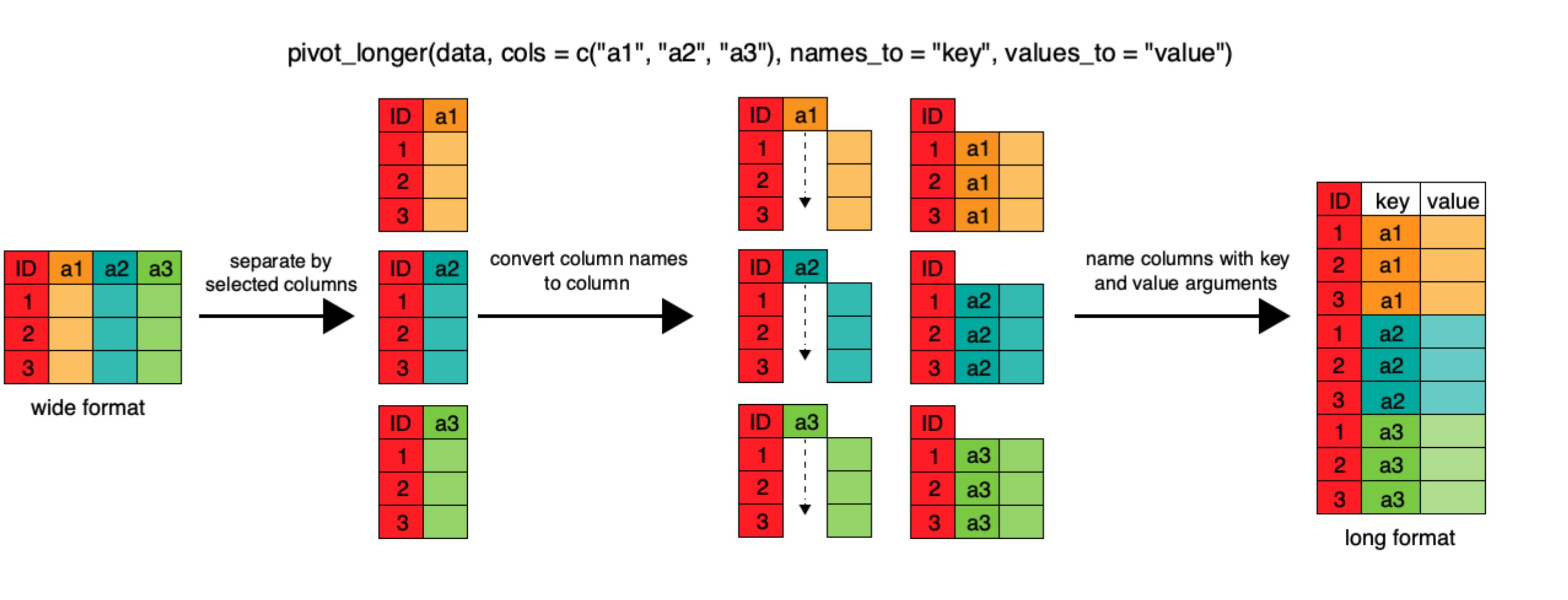
pivot_longer
pivot_longer lengthens data by increasing the
number of rows and decreasing the number of columns. This
function takes 4 main arguments:
- the data
cols, the column(s) to be pivoted (or to ignore)names_tothe name of the new column you’ll create to put the column names invalues_tothe name of the new column to put the column values in
Let’s pretend that we got sent the dataset we just created
(wide_survey) and we want to reshape it to be in a long
format. We can easily do that using pivot_longer
#cols = columns to be pivoted. Here we want to pivot all the plot_id columns, but not the "species_id" column
#names_to = the name of the new column we created from the `cols` argument
#values_to = the name of the new column we will put our values in

surveys_long <- wide_survey %>%
  pivot_longer(cols = -species_id, names_to = "plot_id", values_to = "mean_weight")
This data set should look just like surveys_mz. But this
one is 600 rows, and surveys_mz is 382 rows. What’s going
on?
View(surveys_long)Looks like all the NAs are included in this data set. This is always
going to happen when moving between pivot_longer and
pivot_wider, but is actually a useful way to balance out a
dataset so every replicate has the same composition. Luckily, we now
know how to remove the NAs if we want!
surveys_long <- surveys_long %>%
  filter(!is.na(mean_weight)) #now 382 rows
pivot_wider and pivot_longer are both new
additions to the tidyverse which means there are some cool
new blog posts detailing all their abilities. If you’d like to read more
about this group of functions, check out these links:
Challenge
- Use
pivot_wideron thesurveysdata frame withyearas columns,plot_idas rows, and the number of genera per plot as the values. You will need to summarize before reshaping, and use the functionn_distinct()to get the number of unique genera within a particular chunk of data.
- The
surveysdata set will have two measurement columns:hindfoot_lengthandweight. This makes it difficult to do things like look at the relationship between mean values of each measurement per year in different plot types. Let’s walk through a common solution for this type of problem. First, usepivot_longer()to create a dataset where we have a new column calledmeasurementand avaluecolumn that takes on the value of eitherhindfoot_lengthorweight. Hint: You’ll need to specify which columns are being selected to make longer.
Then with this new data set, calculate the average of eachmeasurementfor each differentplot_type. Then usepivot_wider()to get them into a data set with a column forhindfoot_lengthandweight. Hint: You only need to specify thenames_from =andvalues_from =columns
ANSWER
## Answer 1
surveys <- read_csv("https://ucd-rdavis.github.io/R-DAVIS/data/portal_data_joined.csv")
## Rows: 35549 Columns: 13
## ── Column specification ────────
## Delimiter: ","
## chr (6): species_id, sex, genus, species, taxa, plot_type
## dbl (7): record_id, month, day, year, plot_id, hindfoot_length, weight
##
## ℹ Use `spec()` to retrieve the full column specification for this data.
## ℹ Specify the column types or set `show_col_types = FALSE` to quiet this message.q1 <- surveys %>%
group_by(plot_id, year) %>%
summarize(n_genera = n_distinct(genus)) %>%
pivot_wider(names_from = "year", values_from = "n_genera")## `summarise()` has grouped
## output by 'plot_id'. You can
## override using the `.groups`
## argument.head(q1)## # A tibble: 6 × 27
## # Groups: plot_id [6]
## plot_id `1977` `1978` `1979` `1980` `1981` `1982` `1983` `1984` `1985` `1986`
## <dbl> <int> <int> <int> <int> <int> <int> <int> <int> <int> <int>
## 1 1 2 3 5 7 5 6 7 6 4 3
## 2 2 6 6 6 8 6 9 9 9 6 4
## 3 3 6 7 5 7 7 8 10 11 7 6
## 4 4 4 4 4 4 5 4 6 3 4 3
## 5 5 4 3 3 5 4 6 7 7 3 1
## 6 6 3 5 4 5 5 9 9 7 5 6
## # ℹ 16 more variables: `1987` <int>, `1988` <int>, `1989` <int>, `1990` <int>,
## # `1991` <int>, `1992` <int>, `1993` <int>, `1994` <int>, `1995` <int>,
## # `1996` <int>, `1997` <int>, `1998` <int>, `1999` <int>, `2000` <int>,
## # `2001` <int>, `2002` <int>## Answer 2
q2a <- surveys %>%
pivot_longer(cols = c("hindfoot_length", "weight"), names_to = "measurement_type", values_to = "value")
#cols = columns we want to manipulate
#names_to = name of new column
#values_to = the values we want to fill our new column with (here we already told the function that we were interested in hindfoot_length and weight, so it will automatically fill our new column, which we named "values", with those numbers.)
q2b <- q2a %>%
group_by(measurement_type, plot_type) %>%
summarize(mean_value = mean(value, na.rm=TRUE)) %>%
pivot_wider(names_from = "measurement_type", values_from = "mean_value")## `summarise()` has grouped
## output by 'measurement_type'.
## You can override using the
## `.groups` argument.head(q2b)## # A tibble: 5 × 3
## plot_type hindfoot_length weight
## <chr> <dbl> <dbl>
## 1 Control 32.2 48.6
## 2 Long-term Krat Exclosure 22.5 27.2
## 3 Rodent Exclosure 24.6 32.5
## 4 Short-term Krat Exclosure 27.3 41.2
## 5 Spectab exclosure 33.9 51.6Exporting data
Now that you have learned how to use
dplyr to extract information from or
summarize your raw data, you may want to export these new datasets to
share them with your collaborators or for archival.
Similar to the read_csv() function used for reading CSV
files into R, there is a write_csv() function that
generates CSV files from data frames.
Before using write_csv(), we are going to create a new
folder, data_output, in our working directory that will
store this generated dataset. We don’t want to write generated datasets
in the same directory as our raw data. It’s good practice to keep them
separate. The data folder should only contain the raw,
unaltered data, and should be left alone to make sure we don’t delete or
modify it. In contrast, our script will generate the contents of the
data_output directory, so even if the files it contains are
deleted, we can always re-generate them.
- Type in
write_and hit TAB. Scroll down and take a look at the many options that exist for writing out data in R. Use the F1 key on any of these options to read more about how to use it.