Learning Objectives

Learn the basic date/datetime types in R
Gain familiarity with converting dates and timezones
Learn how to use the lubridate package
Tips and tricks about management of datetime data
Define a function that takes arguments.
Set default values for function arguments.
Explain why we should divide programs into small, single-purpose functions.

Videos

Dates with Lubridate (coming soon)
Function-writing (coming soon)
Video Discussion

In Class Coding

Add a package check/install code block after the YAML header.

Part 1: Date-Times in R

We have learned about different data type classes in previous lessons. Some common data classes we have examined before include character, factor, and numeric. But R also recognizes a data class called “Dates”. Having your date data in the “Dates” data class is very useful, as you can then do things like calculate time between two events, transform the dates into different formats, and plot temporal data easily. In this lesson, we are going to introduce how base R deals with dates (POSIXct or POSITlt), but we are going to spend the majority of our lesson on the package lubridate. lubridate is a great package that makes it much easier to work with dates and times in R.

Date-Time Classes in Base R

Importantly, there are 3 basic time classes in R:

Dates (just dates, i.e., 2012-02-10)
POSIXct (“ct” == calendar time, best class for dates with times)
POSIXlt (“lt” == local time, enables easy extraction of specific components of a time, however, remember that POXIXlt objects are lists)

Unfortunately converting dates & times in R into formats that are computer readable can be frustrating, mainly because there is very little consistency. In particular, if you are importing things from Excel, keep in mind dates can get especially weird¹, depending on the operating system you are working on, the format of your data, etc.

¹ _{For example Excel stores dates as a
number representing days since 1900-Jan-0, plus a fractional portion of
a 24 hour day (serial-time), but in OSX (Mac), it is
1904-Jan-0.}

Dates

The Date class in R can easily be converted or operated on numerically, depending on the interest. Let’s make a string of dates to use for our example:

sample_dates_1 <- c("2018-02-01", "2018-03-21", "2018-10-05", "2019-01-01", "2019-02-18")
#notice we have dates across two years here

What is the class that R classifies this data as?

R classifies our sample_dates_1 data as character data. Let’s transform it into Dates. Notice that our sample_dates_1 is in a nice format: YYYY-MM-DD. This is the format necessary for the function as.Date.

sample_dates_1 <- as.Date(sample_dates_1)

What happens with different orders…say MM-DD-YYYY?

# Some sample dates: 

sample_dates_2 <- c("02-01-2018", "03-21-2018", "10-05-2018", "01-01-2019", "02-18-2019")

sample_dates_3 <-as.Date(sample_dates_2) # well that doesn't work

The reason this doesn’t work is because the computer expects one thing, but is getting something else. Remember, write code you can read and your computer can understand. So we need to give some more information here so R will interpret our data correctly.

# Some sample dates:
sample_dates_2 <- c("02-01-2018", "03-21-2018", "10-05-2018", "01-01-2019", "02-18-2019")

sample_dates_3<- as.Date(sample_dates_2, format = "%m-%d-%Y" ) # date code preceded by "%"

To see a list of the date-time format codes in R, check out this page and table, or you can use: ?(strptime)

The nice thing is this method works well with pretty much any format, you just need to provide the associated codes and structure:

as.Date("2016/01/01", format="%Y/%m/%d")=2016-01-01
as.Date("05A21A2011", format="%mA%dA%Y")=2011-05-21

Challenge

Format this date with the as.Date function: Jul 04, 2019

ANSWER

as.Date("Jul 04, 2019", format = "%b%d,%Y")

## [1] "2019-07-04"

Working with Times in Base R

When working with times, the best class to use in base R is POSIXct.

tm1 <- as.POSIXct("2016-07-24 23:55:26")
tm1

## [1] "2016-07-24 23:55:26 PDT"

tm2 <- as.POSIXct("25072016 08:32:07", format = "%d%m%Y %H:%M:%S")
tm2

## [1] "2016-07-25 08:32:07 PDT"

#Notice how POSIXct automatically uses the timezone your computer is set to. What if we collected this data in a different timezone?

# specify the time zone:
tm3 <- as.POSIXct("2010-12-01 11:42:03", tz = "GMT")
tm3

## [1] "2010-12-01 11:42:03 GMT"

The `lubridate` Package

The lubridate package will handle 90% of the date & datetime issues you need to deal with. It is fast, much easier to work with, and we recommend using it wherever possible. Do keep in mind sometimes you need to fall back on the base R functions (i.e., as.Date()), which is why having a basic understanding of theses functions and their use is important.

To use lubridate we will first need to install and load the package.

#install.packages("lubridate")

library(lubridate)

lubridate has lots of handy functions for converting between date and time formats, and even timezones.

Let’s take a look at our sample_dates_1 data again.

sample_dates_1 <- c("2018-02-01", "2018-03-21", "2018-10-05", "2019-01-01", "2019-02-18")

Once again, R reads this in a character data.

Lubridate uses functions that looks like ymd or mdy to transform data into the class “Date”. Our sample_dates_1 data is formatted like Year, Month, Day, so we would use the lubridate function ymd (y = year, m = month, d = day).

sample_dates_lub <- ymd(sample_dates_1)

What about that messier sample_dates_2 data? Remember R wants dates to be in the format YYYY-MM-DD.

sample_dates_2 <- c("2-01-2018", "3-21-2018", "10-05-18", "01-01-2019", "02-18-2019")
#notice that some numbers for years and months are missing

sample_dates_lub2 <- mdy(sample_dates_2) #lubridate can handle it!

All sorts of date formats can easily be transformed using lubridate:

lubridate::ymd("2016/01/01")=2016-01-01
lubridate::ymd("2011-03-19")=2011-03-19
lubridate::mdy("Feb 19, 2011")=2011-02-19
lubridate::dmy("22051997")=1997-05-22

Using `lubridate` for Time and Timezones

lubridate has very similar functions to handle data with Times and Timezones. To the ymd function, add _hms or _hm (h= hours, m= minute, s= seconds) and a tz argument. lubridate will default to the POSIXct format.

Example 1: lubridate::ymd_hm("2016-01-01 12:00", tz="America/Los_Angeles") = 2016-01-01 12:00:00
Example 2 (24 hr time): lubridate::ymd_hm("2016/04/05 14:47", tz="America/Los_Angeles") = 2016-04-05 14:47:00
Example 3 (12 hr time but converts to 24): lubridate::ymd_hms("2016/04/05 4:47:21 PM", tz="America/Los_Angeles") = 2016-04-05 16:47:21

Lubridate Tips

For lubridate to work, you need the column datatype to be character or factor. The readr package (from the tidyverse) is smart and will try to guess for you. Problem is, it might convert your data for you without the settings (in this case the proper timezone). So here are few ways to work around this.

library(lubridate)
library(dplyr)
library(readr)

# read in some data and skip header lines
nfy1 <- read_csv("https://ucd-rdavis.github.io/R-DAVIS/data/2015_NFY_solinst.csv", skip = 12)
head(nfy1) #R tried to guess for you that the first column was a date and the second a time

## # A tibble: 6 × 5
##   Date       Time      ms Level Temperature
##   <date>     <time> <dbl> <dbl>       <dbl>
## 1 2015-05-22 14:00      0 -8.68           0
## 2 2015-05-22 14:15      0 -8.29           0
## 3 2015-05-22 14:30      0 -8.29           0
## 4 2015-05-22 14:45      0 -8.29           0
## 5 2015-05-22 15:00      0 -8.30           0
## 6 2015-05-22 15:15      0 -8.29           0

# import raw dataset & specify column types
nfy2 <- read_csv("https://ucd-rdavis.github.io/R-DAVIS/data/2015_NFY_solinst.csv", col_types = "ccidd", skip=12)

glimpse(nfy1) # notice the data types in the Date.Time and datetime cols

## Rows: 7,764
## Columns: 5
## $ Date        <date> 2015-05-22, 2015-05-22, 2015-05-22, 2015-05-22, 2015-05-2…
## $ Time        <time> 14:00:00, 14:15:00, 14:30:00, 14:45:00, 15:00:00, 15:15:0…
## $ ms          <dbl> 0, 0, 0, 0, 0, 0, 0, 0, 0, 0, 0, 0, 0, 0, 0, 0, 0, 0, 0, 0…
## $ Level       <dbl> -8.6834, -8.2928, -8.2914, -8.2901, -8.2955, -8.2935, -8.2…
## $ Temperature <dbl> 0, 0, 0, 0, 0, 0, 0, 0, 0, 0, 0, 0, 0, 0, 0, 0, 0, 0, 0, 0…

glimpse(nfy2)

## Rows: 7,764
## Columns: 5
## $ Date        <chr> "2015/05/22", "2015/05/22", "2015/05/22", "2015/05/22", "2…
## $ Time        <chr> "14:00:00", "14:15:00", "14:30:00", "14:45:00", "15:00:00"…
## $ ms          <int> 0, 0, 0, 0, 0, 0, 0, 0, 0, 0, 0, 0, 0, 0, 0, 0, 0, 0, 0, 0…
## $ Level       <dbl> -8.6834, -8.2928, -8.2914, -8.2901, -8.2955, -8.2935, -8.2…
## $ Temperature <dbl> 0, 0, 0, 0, 0, 0, 0, 0, 0, 0, 0, 0, 0, 0, 0, 0, 0, 0, 0, 0…

Next we want to create a single datetime column. How do we get our Date and Time columns into one column so we can format it as a datetime? The answer is the paste function.

paste() allows pasting text or vectors (& columns) by a given separator that you specify with the sep = argument
paste0() is the same thing, but defaults to using no separator (i.e. no space).

# make a datetime col:
nfy2$datetime <- paste(nfy2$Date, " ", nfy2$Time, sep = "")

glimpse(nfy2) #notice the  datetime column is classifed as character

## Rows: 7,764
## Columns: 6
## $ Date        <chr> "2015/05/22", "2015/05/22", "2015/05/22", "2015/05/22", "2…
## $ Time        <chr> "14:00:00", "14:15:00", "14:30:00", "14:45:00", "15:00:00"…
## $ ms          <int> 0, 0, 0, 0, 0, 0, 0, 0, 0, 0, 0, 0, 0, 0, 0, 0, 0, 0, 0, 0…
## $ Level       <dbl> -8.6834, -8.2928, -8.2914, -8.2901, -8.2955, -8.2935, -8.2…
## $ Temperature <dbl> 0, 0, 0, 0, 0, 0, 0, 0, 0, 0, 0, 0, 0, 0, 0, 0, 0, 0, 0, 0…
## $ datetime    <chr> "2015/05/22 14:00:00", "2015/05/22 14:15:00", "2015/05/22 …

# convert Date Time to POSIXct in local timezone using lubridate
nfy2$datetime_test <- as_datetime(nfy2$datetime, 
                                    tz="America/Los_Angeles")
# OR convert using the ymd_functions
nfy2$datetime_test2 <- ymd_hms(nfy2$datetime, tz="America/Los_Angeles")

# OR wrap in as.character()
nfy1$datetime <- ymd_hms(as.character(paste0(nfy1$Date, " ", nfy1$Time)), tz="America/Los_Angeles")
tz(nfy1$datetime)

## [1] "America/Los_Angeles"

Last, lubridate lets you extract components of date, time and datetime data types with intuitive functions.

# Functions called day(), month(), year(), hour(), minute(), second(), etc... will extract those elements of a datetime column.
months <- month(nfy2$datetime)
# Use the table function to get a quick summary of categorical variables
table(months)

## months
##    5    6    7    8 
##  904 2880 2976 1004

# Add label and abbr agruments to convert numeric representations to have names
months <- month(nfy2$datetime, label = TRUE, abbr=TRUE)
table(months)

## months
##  Jan  Feb  Mar  Apr  May  Jun  Jul  Aug  Sep  Oct  Nov  Dec 
##    0    0    0    0  904 2880 2976 1004    0    0    0    0

Part 2: Creating Functions

Any operation you will perform more than once can be put into a function. That way, rather than retyping all the commands (and potentially making errors), you can simply call the function, passing it a new dataset or parameters. This may seem cumbersome at first, but writing functions to automate repetitive tasks is incredibly powerful. E.g. each time you call ggplot you are calling a function that someone wrote. Imagine if each time you wanted to make a plot you had to copy and paste or write that code from scratch!

Defining a function

Recall the components of a function. E.g. the log function (see ?log) takes “arguments” x and base and “returns” the base-base logarithm of x. Functions take arguments as input and yield return-values as output. You can define functions to do any number of operations on any number of arguments, but always output a single return value (however there are complex objects into which you can put multiple objects, should you need to).

Let’s start by defining a simple function to add two numbers. This is the basic structure, which you can read as “assign to the variable my_sum a function that takes arguments a and b and returns the_sum.” The body of the function is delimited by the curly-braces. The statements in the body are indented. This makes the code easier to read but does not affect how the code operates.

my_sum <- function(a, b) {
  the_sum <- a + b
  return(the_sum)
}

Notice that no numbers were summed when we ran that code, but now the Environment has an object called my_sum that has type function. You can call my_sum just like you would any other function. When you do, the code between the curly-braces of the my_sum definition is run with whatever values you pass to a and b substituted in their place.

my_sum(a = 2, b = 2)

## [1] 4

my_sum(3, 4)

## [1] 7

Just like log provides a default value of base (exp(1)) so that you don’t have to type it every time, you can provide default values to any arguments of your function. Then if the user doesn’t specify them, the defaults will be used.

my_sum2 <- function(a = 1, b = 2) {
  the_sum <- a + b
  return(the_sum)
}
my_sum2()

## [1] 3

my_sum2(b = 7)

## [1] 8

Tip

One feature unique to R is that the return statement is not required. R automatically returns the output of the last line of the body of the function unless a return statement is specified elsewhere. Since other languages require a return statement and because it can make reading a function easier, we will explicitly define the return statement.

Temperature conversion

Let’s define a function F_to_K that converts temperatures from Fahrenheit to Kelvin:

F_to_K <- function(temp) {
  K <- ((temp - 32) * (5 / 9)) + 273.15
  return(K)
}

Calling our own function is no different from calling any other function:

# freezing point of water
F_to_K(32)

## [1] 273.15

# boiling point of water
F_to_K(212)

## [1] 373.15

Challenge

Write a function called K_to_C that takes a temperature in K and returns that temperature in C
- Hint: To convert from K to C you subtract 273.15
Create a new R script, copy F_to_K and K_to_C in it, and save it as functions.R in the code directory of your project.

ANSWER

K_to_C <- function(tempK) {
    tempC <- tempK - 273.15 
    return(tempC)
}

`source()`ing functions

You can load all the functions in your code/functions.R script without even opening the file, via the source function. This allows you to keep your functions separate from the analyses which use them.

source('code/functions.R')

Using dataframes in functions

Let’s write a function to calculate the average GDP in a given country, in a given span of years, based on the gapminder data. If you were to do this for just one specification, without writing a function, it might look something like this:

library(gapminder)

## 
## Attaching package: 'gapminder'

## The following object is masked _by_ '.GlobalEnv':
## 
##     gapminder

library(tidyverse)

gapminder %>% 
  filter(country == "Canada", year %in% c(1950:1970)) %>% 
  summarize(mean(gdpPercap, na.rm = T))

## # A tibble: 1 × 1
##   `mean(gdpPercap, na.rm = T)`
##                          <dbl>
## 1                       13349.

But, what if you wanted to do this for many different specifications? You might find yourself wanting to copy and paste these couple lines of code over and over. Instead, you can write it into a function, soft coding the parts that you want as your function’s arguments. In this example, we want to be able to change the country and the year range that we are interested in.

# Note: try to name arguments something that do not exist as a column name, to avoid confusing yourself and R
avgGDP <- function(cntry, yr.range){
  df <- gapminder %>% 
  filter(country == cntry, year %in% yr.range)
  mean(df$gdpPercap, na.rm = T)
}

avgGDP("Iran", 1980:1985)

## [1] 7608.335

avgGDP("Zimbabwe", 1950:2000)

## [1] 648.8549

Pass by value

Functions in R almost always make copies of the data to operate on inside of a function body. When we modify a data frame inside the function we are modifying the copy of the gapminder dataset, not the original variable we gave as the first argument. This is called “pass-by-value” and it makes writing code much safer: you can always be sure that whatever changes you make within the body of the function, stay inside the body of the function.

Challenge

This challenge will deal with countries’ population growth. To access the data, load (and install, if needed) the gapminder library and access its life expectancy dataset using:

library(gapminder)
d <- gapminder::gapminder

Write a new function that takes two arguments, the gapminder data.frame (d) and the name of a country (e.g. "Afghanistan"), and plots a time series of the country’s population. The return value from the function should be a ggplot object. Note: It is often easier to modify existing code than to start from scratch. To start out with one plot for a particular country, figured out what you need to change for each iteration (these will be your arguments), and then wrap it in a function.

ANSWER

plotPopGrowth <- function(countrytoplot, dat = gapminder) {
    df <- filter(dat, country == countrytoplot) 
    plot <- ggplot(df, aes(year, pop)) + 
        geom_line()
    return(plot)
}
plotPopGrowth('Canada')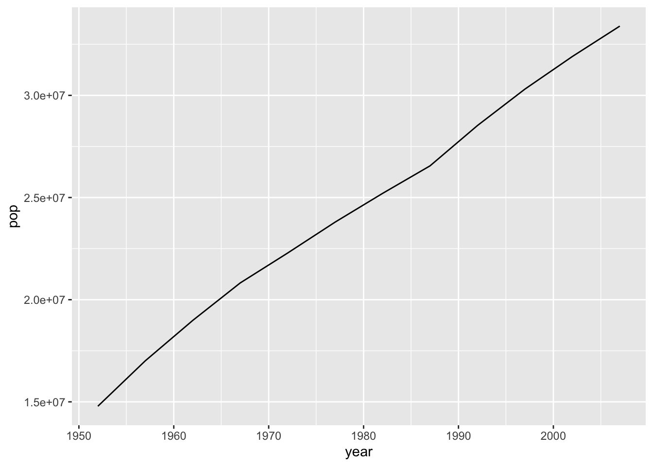

This lesson was contributed by Ryan Peek and Martha Zillig.

This lesson is adapted from the Software Carpentry: R for Reproducible Scientific Analysis Creating Functions materials.

Wk08: Dates & Times with Lubridate and Creating Functions

Working with datetimes and writing your own functions

Learning Objectives

Videos

In Class Coding

Add a package check/install code block after the YAML header.

Part 1: Date-Times in R

Date-Time Classes in Base R

Dates

Challenge

Working with Times in Base R

The `lubridate` Package

Using `lubridate` for Time and Timezones

Lubridate Tips

Part 2: Creating Functions

Defining a function

Tip

Temperature conversion

Challenge

`source()`ing functions

Using dataframes in functions

Pass by value

Challenge

Wk08: Dates & Times with Lubridate and Creating Functions

Working with datetimes and writing your own functions

Learning Objectives

Videos

In Class Coding

Add a package check/install code block after the YAML header.

Part 1: Date-Times in R

Date-Time Classes in Base R

Dates

Challenge

Working with Times in Base R

The lubridate Package

Using lubridate for Time and Timezones

Lubridate Tips

Part 2: Creating Functions

Defining a function

Tip

Temperature conversion

Challenge

source()ing functions

Using dataframes in functions

Pass by value

Challenge

The `lubridate` Package

Using `lubridate` for Time and Timezones

`source()`ing functions